Axon: The STICK Software Development Kit
The brain, a truly efficient computation machine, encodes and processes information using discrete spikes. Inspired by this, we’ve built Axon, a neuromorphic software framework for building, simulating, and compiling Spiking Neural Networks (SNNs) for general-purpose computation. Axon allows to build complex computation by combining modular computation kernels, avoiding the challenge of having to train case-specific SNN while maintaining the sparsity of spike computing.
Axon is an extension of STICK (Spike Time Interval Computational Kernel).
The code is open-source on Gihub > Axon SDK
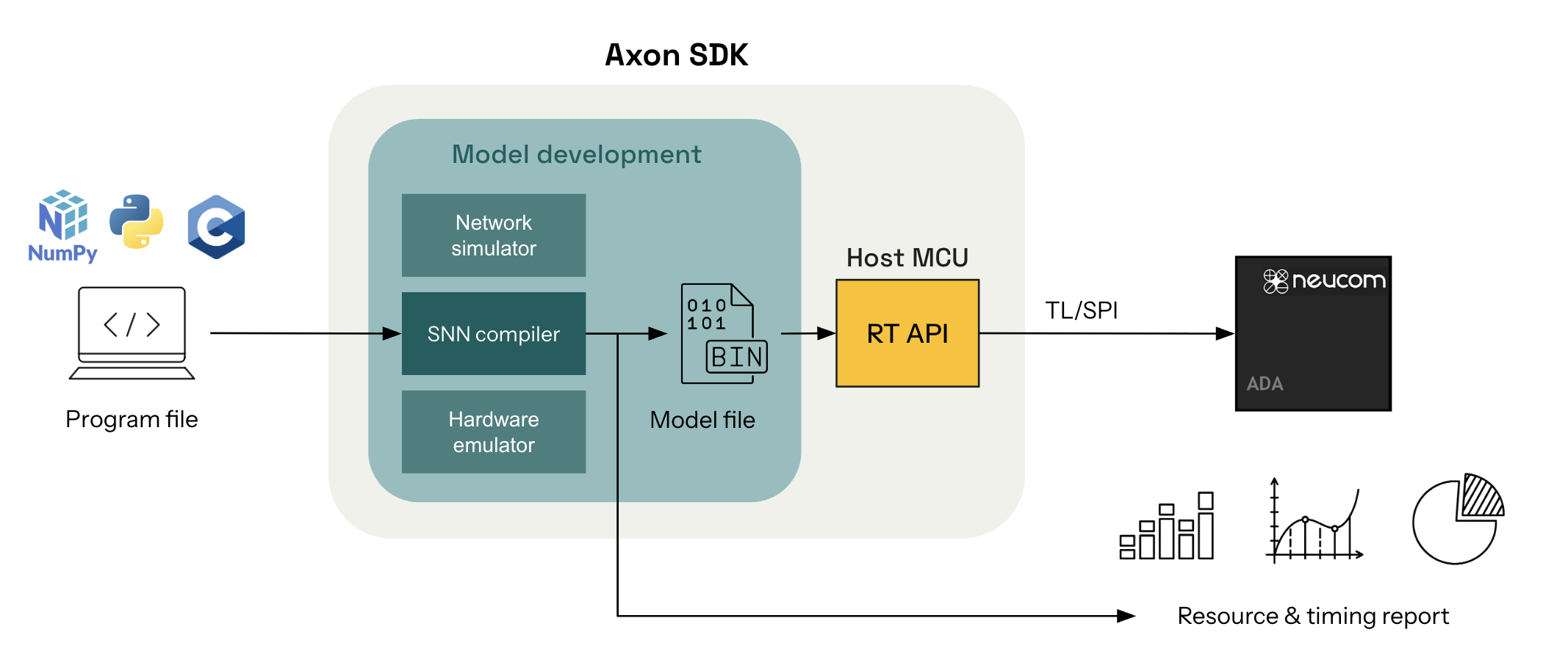
Axon provides an end-to-end pipeline for deploying deterministic algorithms as interval-coded SNNs to ultra-low-power neuromorphic hardware.
At Neucom, we’re building one of such neuromorphic chips and we’re calling it ADA. ADA aims to marry together the low-power consumption of FPGAs and ASICS while keeping the flexibility and ease of use of microcontrollers.
The Axon SDK includes:
- A SNN simulator for accurate emulation of the interval-coded symbolic computation.
- A compiler for translating Python-defined algorithms into spiking circuits, ready for simulation or deployment.
- Resource reporting tools for latency estimation and performance profiling of the deployed algorithms.
If you’re building symbolic SNNs for embedded inference, signal processing, control, or cryptographic tasks, Axon makes it easy to translate deterministic computations into spiking neural networks.
Axon SDK structure
| Component | Description |
|---|---|
axon_sdk.primitives | Base clases defining the low level components and engine used by the spiking networks |
axon_sdk.networks | Library of modular spiking computation kernels |
axon_sdk.simulator | Spiking network simulator to input spikes, simulate dynamics and read outputs |
axon_sdk.compilation | Compiler for transforming high-level algorithms into spiking networks |
Example: Float multiplication SNN
from axon_sdk.simulator import Simulator
from axon_sdk.networks import MultiplierNetwork

encoder = DataEncoder(Tmin=10.0, Tcod=100.0)
net = MultiplierNetwork(encoder)

val1 = 0.1
val2 = 0.5

sim = Simulator(net, encoder, dt=0.01)

# Apply both input values
sim.apply_input_value(val1, neuron=net.input1, t0=10)
sim.apply_input_value(val2, neuron=net.input2, t0=10)

# Simulate long enough to see output
sim.simulate(simulation_time=400)

spikes = sim.spike_log.get(net.output.uid, [])
interval = spikes[1] - spikes[0]
decoded_val = encoder.decode_interval(interval)
decoded_val
>> 0.05
Citation
If you use Axon in your research, please cite:
@misc{axon2025,
  title        = {Axon: A Software Development Kit for Symbolic Spiking Networks},
  author       = {Neucom},
  howpublished = {\url{https://github.com/neucom/axon}},
  year         = {2025}
}
License
The Axon SDK is open-sourced under a GPLv3 license, preventing by default its inclusion in closed-source projects. However, reach out to initiate a collaboration if you’d like to incorporate Axon into your closed-source project.
![]()
Getting Started
Installation
The Axon SDK can be installed from its source code. which is open-sourced on Github.
git clone https://github.com/neucom/axon-sdk.git
cd axon-sdk
pip install -e .
The Axon SDK is built in Python and depends on:
- Python ≥ 3.11
- NumPy
- Matplotlib
- Pytest
The dependencies can be installed using the requirements file:
cd axon-sdk
pip install -r requirements.txt
Quickstart
This tutorial will showcases how to use Axon to build a Spiking Neural Network (SNN) that can multiply two signed decimal numbers. In particular, it covers how to use a multiplication SNN module available in Axon, how input values to it, how simulate its execution, and how to read out and interpret the output.
Multiplier and encoder
The spiking neural networks (SNN) defined with Axon SDK are slightly different from what’s conventionally understood by spiking neural networks (for example, in ML). They have two fundamental differences:
- Axon’s SNNs don’t need to be trained.
- Axon uses a pair of spikes to encode an individual value.
The Axon SDK provides an already-made library of computational modules. These are SNNs implementing a specific and deterministic computation.
One of such modules is a multiplication network:
from axon_sdk.networks import MultiplierNetwork
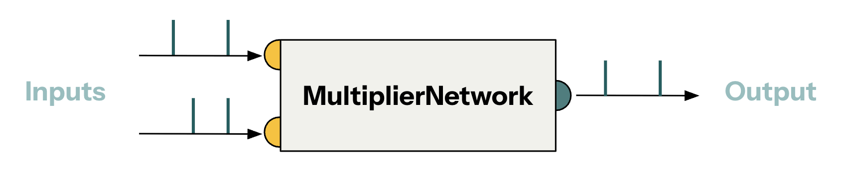
Axon abstracts the complexity of the underlying SNNs into a modular interface that allows composing computation kernels to achieve larger operations.
The multiplier network requires an encoder to work. The encoder is the component that translates between arithmetic values and spike intervals.
from axon_sdk.primitives import DataEncoder

encoder = DataEncoder(Tmin=10.0, Tcod=100.0)

spikes = enc.encode_value(0.2)
interval = spikes[1] - spikes[0]
value = enc.decode_interval(interval)
spikes
>> (0, 30.0)

value
>> 0.2
Simulating the SNN
There is one last fundamental ingredient to execute the SNN - the simulator:
from axon_sdk.primitives import Simulator

sim = Simulator(multiplier_net, encoder, dt=0.01)
The simulator runs a sequential execution of the dynamics of the SNN, hence the need of a simulation timestep parameter (dt).
The simulator also allows to input values to the network. Under the hood, it uses the encoder to do so:
sim.apply_input_value(0.5, neuron=net.input1)
sim.apply_input_value(0.5, neuron=net.input2)
The last step is to run the simulation and to readout the spikes emitted by the output neuron
sim.simulate(simulation_time=400)
spikes = sim.spike_log.get(net.output.uid, [])

interval = spikes[1] - spikes[0]
output_val = encoder.decode_interval(interval)
output_val
>> 0.2
Instead of using spiking rates to encode values which encode values over many spikes, Axon uses inter-spike intervals. The delay betweekn a couple of spikes encodes a value. This makes Axon extremely spike sparse, hence optimizing for energy consumption (when deploying spiking neural networks to hardware, processing each spike has an energy cost)
Tutorials
Combining computations
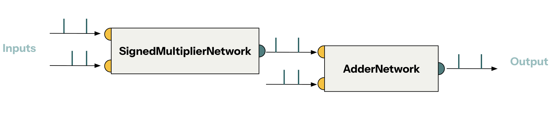
Axon SDK provides a library of modular spiking computation kernels that can be combined to achieve complex computations. In this tutorial, we will build a Spiking Multiply-Accumulate module by combining primitive modules.
Spiking Multiply-Accumulate (MAC)
A multiply-accumulate computation over signed scalars takes the following form:
y = a * x + b
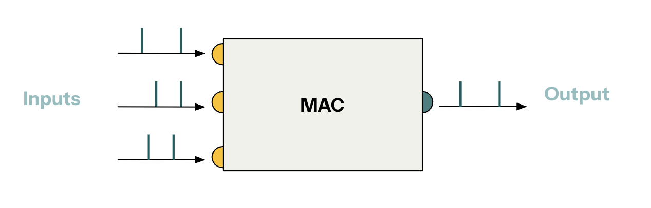
Axon provides spiking modules to implement signed multiplication and addition as part of its library. Combining them, we can build a MAC module.
| Module | Description |
|---|---|
SignedMultiplierNetwork | Multiplies two signed scalars |
AdderNetwork | Adds two signed scalars |
Combining modules requires wiring them together. We will see how to wire the modules together later on.
Signed channels in spiking modules
Signed arithmetics is achieved by having two channels per input/output (one channel for each sign). Therefore, pair of spikes in a certain channel encodes a signed value.
Each module that supports signed arithmetics contains two neurons per input/output:
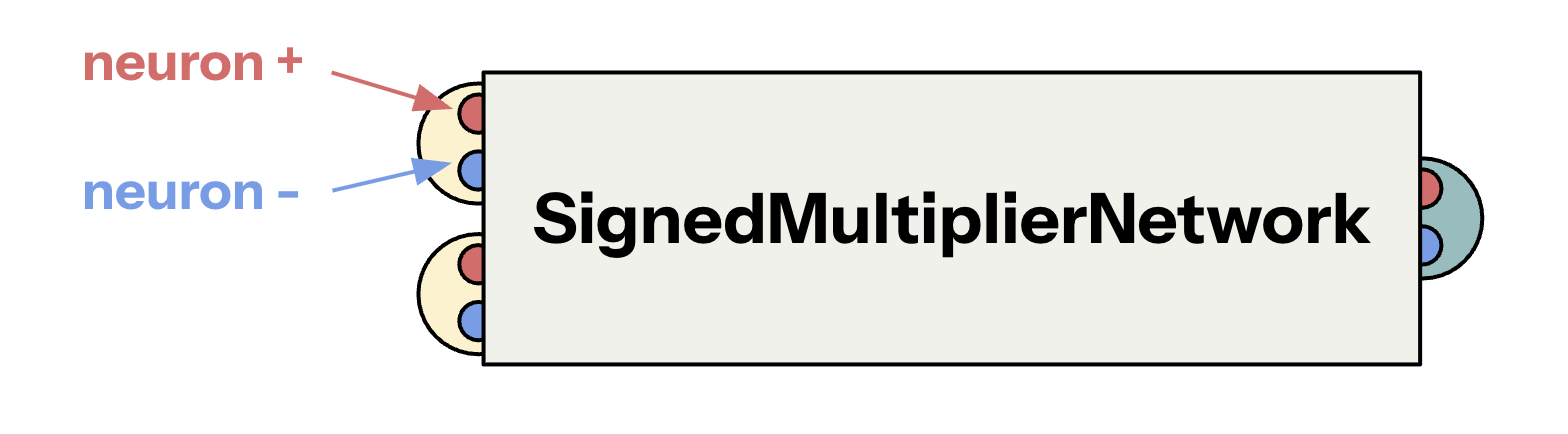
| Module | Inputs | Outputs |
|---|---|---|
SignedMultiplierNetwork | net.input1_plus | net.output1_plus |
net.input1_minus | net.output1_minus | |
net.input2_plus | ||
net.input2_minus | ||
AdderNetwork | net.input1_plus | net.output1_plus |
net.input1_minus | net.output1_minus | |
net.input2_plus | ||
net.input2_minus |
Wiring modules together
Putting together the MAC module is a matter of wiring together the SignedMultiplierNetwork and AdderNetwork, making sure to wire plus to plus and minus to minus.
from axon_sdk.networks import SignedMultiplierNetwork, AdderNetwork
from axon_sdk.primitives import SpikingNetworkModule

class MacNetwork(SpikingNetworkModule):
    def __init__(self, encoder):
        super().__init__()

        we = 10.0
        Tsyn = 1.0

        self.add_net = AdderNetwork(encoder)
        self.mul_net = SignedMultiplierNetwork(encoder)

        self.connect_neurons(self.mul_net.output_plus,
            self.add_net.input1_plus,
            synapse_type="V",
            weight=we,
            delay=Tsyn
        )
        self.connect_neurons(self.mul_net.output_minus,
            self.add_net.input1_minus,
            synapse_type="V",
            weight=we,
            delay=Tsyn
        )

        self.add_subnetwork(add_net)
        self.add_subnetwork(mul_net)
Defining the new MAC module, or any new module, requires subclassing SpikingNetworkModule. This base class does basic housekeeping (e.g. making sure each child module has a unique ID, etc.)
Note: The call to
self.add_subnetwork(...)is important. It’s required for the base class to register the new module as a child. Without it, the simulation of the dynamics (which we’ll do later on) will not work properly.
There are several things to explain from the snippet above: the origin of the values we, Tsyn and V:
The variable we stands for weight excitatory and it’s a term used throught Axon. It’s the weigth of a synapse that will excite (trigger) the following neuron in a single timestep. Using we=10.0 comes from the fact that neurons, usually, have a voltage threshold Vt=10, defined in each module (look inside signed_multiplier.py).
The variable Tsyn stands for synapse time and using it’s the time delay introduced by the synapse. The value Tsyn=1.0 is used by default throughtout Axon. It’s arbitrary and can be changed without affecting the dynamics of the spiking networks.
The synapses used to connect the modules are of type V. V-synapses cause the following network to spike right after receiving a spike. Hence, they are used to propagate information forward in the network.
The simulator
In order to make the network spike, we need some sort of engine that handles the simulation of the dynamics of the spikes. That engine is the Simulator.
from axon_sdk.simulator import Simulator
from axon_sdk.primitives import DataEncoder

encoder = DataEncoder(Tmin=10.0, Tcon=100.0)

mac_net = MacNetwork(encoder)
sim = Simulator(mac, encoder, dt=0.01)
For an explanation about how DataEncoder encodes values, take a look at Core concepts > Interval coding
The simulator evolves the spiking module sequentially with a timestep of dt. Using dt=0.01 is enough to get accurate simulations for most networks. In some cases, dt=0.001 is also used. In general, we want dt << Tsyn.
Inputs & outputs
The simulator is in charge of inputting spikes to the network.
Let’s set some numeric values for the MAC operation:
a = 0.5
x = 0.3
b = 0.8
Using those:
y = a * x + b = 0.95
We can use the simulator’s method .apply_input_value(val, neuron, t) to input spikes to the network.
a = 0.5
x = 0.3
b = 0.8

sim.apply_input_value(a, mac_net.mul_net.input1_plus, t0=0)
sim.apply_input_value(x, mac_net.mul_net.input2_plus, t0=0)
sim.apply_input_value(b, mac_net.add_net.input2_plus, t0=0)
The method Simulator.apply_input_value(val, neuron, t) automatically applies a couple of spikes encoding a value to a neuron at a timestep t. To input an individual spike, there is also Simulator.apply_input_spike(neuron, t).
Since in this example all inputs are positive, we can manually input them to the plus neurons. Inputing values manually is an academic exercise which does not scale to real-world scenatios. In further tutorials we’ll see how to automate this process.
Running the simulation
Now, it’s just a matter of letting the simulation run for a certain amount of time:
sim.simulate(simulation_time=500)
If everything went fine, the plus output of the adder module should have spiked twice, and the interval between the spikes will encode the desired value - 0.95.
spikes_plus = sim.spike_log.get(mac_net.add_net.output_plus.uid, [])
spikes_plus
>> [381.94, 486.94]
encoder.decode_interval(spikes_plus[1] - spikes_plus[0])
>> 0.95
Using the computation compiler
So far, we have combined manually different computational blocks to achieve a larger computation (for example, in the tutorial Combining computations). However, that becomes unfeasible when wanting to run larger computations or even full algorithms.
Axon SDK provides a computation compiler that translates a computation defined in Python to its corresponding spiking network, which implements such computation. The goal of this tutorial is to introduce the computation compiler.
The Scalar class
Axon SDK provides a class whose purpose is to track the computations applied to scalar values. That class is called Scalar.
The Scalar base class wraps floating-point scalars with the purpose of logging the operations performed over them during algorithms.
from axon_sdk.compilation import Scalar

a = Scalar(0.5)
x = Scalar(0.3)
b = Scalar(0.8)
The Axon compiler works by logging the subsequent computations performed over scalars, building a computation graph and finally, transforming it into its equivalent spiking network.
After the variables are tracked by a Scalar, we can use them as we would in normal Python syntax to implement algorithms:
y_mac = a * x + b
We can also visualize the built computation graph:
y_mac.draw_comp_graph(outfile='MAC_computation_graph')
The computation graph is a graphical representation of a computation where each node represents an operation and each edge a scalar value.
It’s possible to use more complex computations over variables wrapped by Scalar. Everything works as expected:
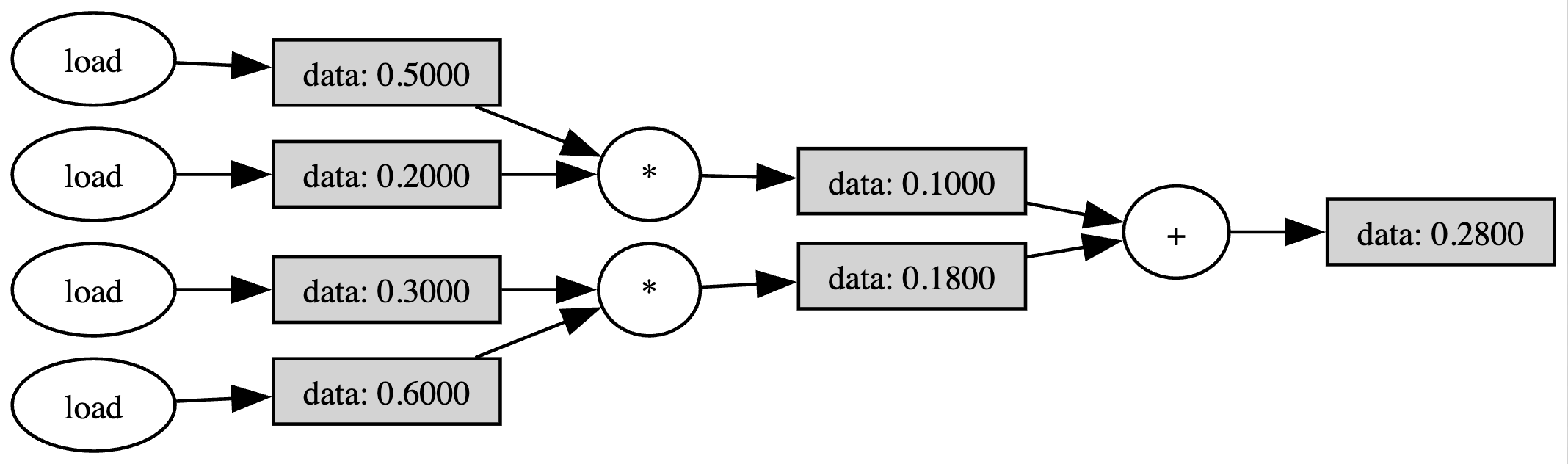
from axon_sdk.compilation import Scalar

def dot_prod(a: list[Scalar], b: list[Scalar]):
    return a[0] * b[0] + a[1] * b[1]

a = [Scalar(0.5), Scalar(0.3)]
b = [Scalar(0.2), Scalar(0.6)]

y_dot = dot_prod(a, b)
y_dot.draw_comp_graph(outfile='dot_computation_graph')
Once we have a computational graph built, we can transform it into a spiking network using the compiler.
From computation graph to spiking network
Axon provides a compilation module with methods for performing the compilation process and objects to hold the output of the compilation. The compile_computation() method transforms a computation graph to a spiking network:
from axon_sdk.compilation import ExecutionPlan, compile_computation
from axon_sdk.compilation import Scalar

a = Scalar(0.5)
x = Scalar(0.3)
b = Scalar(0.8)

y = a * x + b

exec_plan = compile_computation(y, max_range=1)
Note: Since our variables in this example are bounded by 1, we can use a
max_range=1. Using a larger range allows to perform computations with an extended numeric range, but that comes at a cost of precision when executing the spiking network.
The output of the compilation process is an ExecutionPlan.
ExecutionPlan
 | net
 | triggers
 | reader
The execution plan contains the generated spiking network in net. Besides, it contains triggers objects that automatically handle the process of inputting data to the spiking net (taking care of value range normalization and sign) and reader, for reading the output of the network.
The execution plan is ready to be simulated:
Simulating the spiking computation
The simulator knows how to run the execution plan produced by the compilation:
from axon_sdk.simulator import Simulator

encoder = DataEncoder(Tmin=10.0, Tcod=100.0)

sim = Simulator.init_with_plan(exec_plan, enc)
sim.simulate(simulation_time=600)
All that is left is to readout the output spikes and decode the value
spikes_plus = sim.spike_log.get(execPlan.output_reader.read_neuron_plus.uid, [])
spikes_plus
>> [381.94, 486.94]

encoder.decode_interval(spikes_plus[1] - spikes_plus[0])
>> 0.95
As expected, the spiking network outputs spikes that, when decoded, have computed 0.5 * 0.3 + 0.8 = 0.95.
Supported operations
The current version of the compiler supports the following scalar operations:
| Operation | Description |
|---|---|
ADD | a + b |
NEG | - b |
MUL | a * b |
DIV | a / b |
Only algorithms that use the Python operators +, -, * and \ can be compiled to spiking networks.
Other primitive arithmetic operations (EXP, etc.), complex operations (RELU, etc.) and control flow operations (BEQ, etc.) will be added in future releases.
Feel free to submit requests to extend the supported operations in our Github issues.
Using an extended numerical range
In the example before, the input variables were bounded by 1. Both the input values and any intermediate value had to be in the range [-1, 1].
Important: It’s the users responsability to guarantee that any input value and intermediate computation value is in the range
[-1, 1]. The current version of the compiler does not detect overflows. Failure to comply to this will yield an unreliable spiking execution.
However, we can use an extended numerical range which grants more computational freedom by adjusting max_range:
a = Scalar(5)
x = Scalar(3)
b = Scalar(8)

y = a * x + b

exec_plan = compile_computation(y, max_range=100)
It’s still the user’s responsability to guarantee that the input and intermediate values are within [-max_range, max_range].
Behind the scenes, both the simulator and the spiking network are reconfigured to take care of the extended numeric range. Inputs are linearly squeezed to [-1, 1] and intermediate operations compensate the normalization constant.
For example, multiplications must compensate for an extra max_range in the denominator:
a * b -> (a / max_range) * (b / max_range) -> a * b / (max_range)^2
From a user’s perspective, everything behaves as expected:
encoder = DataEncoder(Tmin=10.0, Tcod=100.0)

sim = Simulator.init_with_plan(exec_plan, enc)
sim.simulate(simulation_time=600)

spikes_plus = sim.spike_log.get(exec_plan.output_reader.read_neuron_plus.uid, [])
The only difference is that, now, the readout value must be de-normalized:
decoded_val = enc.decode_interval(spikes_plus[1] - spikes_plus[0])
de_norm_value = decoded_val * exec_plan.output_reader.normalization
de_norm_value
>> 23
Building custom spiking modules
In other tutorials, we have used the spiking modules provided by the Axon SDK library or combined them to define complex computations. However, in certain cases one might need to define modules from scratch. Axon SDK provides an infrastructure to do that.
In this tutorial, we will implement from scratch a module that computes the minimum between two input values. This is, a MinNetwork module, which is not part of the Axon library (yet).
MinNetwork: compute the minimum
Axon is based on the theoretical foundation introduced by the STICK framework, presented in the paper STICK: Spike Time Interval Computational Kernel, A Framework for General Purpose Computation using Neurons, Precise Timing, Delays, and Synchrony. In the paper, there is a design for a spiking network that computes the minimum between two floating point values, which is the one we will implement in this tutorial.
Note: For a deep understanding of the operating principles behind STICK and the workings of the minimum network, the STICK paper contains a great explanation. If you’re interested in learning about it, please, refer to the paper. This tutorial will only address the implementation and simulation of the network in Axon.
This is the spiking network presented in the paper to compute the minimum between two inputs:
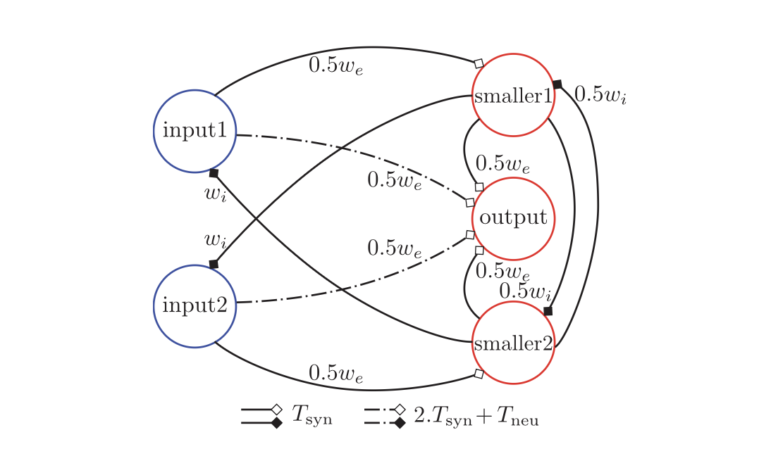
Let’s break down the meaning of the graph, step by step.
Each node represents a spiking neuron and each edge, a synaptic connection.
Each synapse has 3 parameters which define it’s properties:
Synapse
 | - type
 | - weight
 | - delay
All synapses are black and therefore V-type synapses (as presented in the paper).
The weight of each synapse is plotted by it. We can see the values we, wi and combinations of them with a preceding factor. The weight we stands for weight excitatory and means that a synapse with weight we will cause the receiving neuron to spike immediately (in the next update cycle). The wi stands for weight inhibitory and has the contrary effect: After receiving a wi synapse, a neuron will need 2x we to spike.
The delays of the synapses, indicated by the line type, have the values Tsyn and Tsyn + Tneu. The first, Tsyn, stands for synapse time and it’s an arbitrary but constant value, usually set to Tsyn=1. The second, Tneu stands for neuron propagation time and is the time a neuron takes to spike after its membrane potential went over the spiking threshold. Since we’re using a sequential simulator, Tneu = dt.
Presenting the SpikingNetworkModule
All spiking modules must be childs of a base class called SpikingNetworkModule. Creating new modules requires subclassing it as well.
from axon_sdk.primitives import SpikingNetworkModule

class MinNetwork(SpikingNetworkModule):
    def __init__(self, encoder, module_name=None):
        super().__init__(module_name)
        ...
The SpikingNetworkModule does basic housekeeping: keeps track of child submodules and neurons, makes sure submodules have unique IDs, and provides methods to wire larger modules together. In short, it allows modularity and composability when building complex spiking networks.
Building the Minimum Network
We can follow the graph describin the minimum network from the STICK paper and wire a new spiking module:
class MinNetwork(SpikingNetworkModule):
    def __init__(self, encoder, module_name='min_network'):
        super().__init__(module_name)

        # neuron params
        Vt = 10.0  # threshold voltage
        tm = 100.0
        tf = 20.0

        # synapse params
        we = Vt
        wi = -Vt
        Tsyn = 1.0
        Tneu = 0.01

        self.input1 = self.add_neuron(Vt, tm, tf, neuron_name='input1')
        self.input2 = self.add_neuron(Vt, tm, tf, neuron_name='input2')
        self.smaller1 = self.add_neuron(Vt, tm, tf, neuron_name='smaller1')
        self.smaller2 = self.add_neuron(Vt, tm, tf, neuron_name='smaller2')
        self.output = self.add_neuron(Vt, tm, tf, neuron_name='output')

        # from input1
        self.connect_neurons(self.input1, self.smaller1, "V", 0.5 * we, Tsyn)
        self.connect_neurons(self.input1, self.output, "V", 0.5 * we, 2 * Tsyn + Tneu)

        # from input2
        self.connect_neurons(self.input2, self.smaller2, "V", 0.5 * we, Tsyn)
        self.connect_neurons(self.input2, self.output, "V", 0.5 * we, 2 * Tsyn + Tneu)

        # from smaller1
        self.connect_neurons(self.smaller1, self.input2, "V", wi, Tsyn)
        self.connect_neurons(self.smaller1, self.output, "V", 0.5 * we, Tsyn)
        self.connect_neurons(self.smaller1, self.smaller2, "V", 0.5 * wi, Tsyn)

        # from smaller2
        self.connect_neurons(self.smaller2, self.input1, "V", wi, Tsyn)
        self.connect_neurons(self.smaller2, self.output, "V", 0.5 * we, Tsyn)
        self.connect_neurons(self.smaller2, self.smaller1, "V", 0.5 * wi, Tsyn)
Once built, we can use the simulator to run the dynamics of the network. Refer to the tutorial on Combining computations for a longer explanation about the simulator.
from axon_sdk.simulator import Simulator
from axon_sdk.primitives import DataEncoder

encoder = DataEncoder(Tmin=10.0, Tcod=100.0)
min_net = MinNetwork(encoder, 'min')
sim = Simulator(min_net, encoder)
What’s the smaller value between 0.7 and 0.2? That’s a hard question. Let’s find it out:
val1 = 0.7
val2 = 0.2

sim.apply_input_value(val1, min_net.input1, t0=0)
sim.apply_input_value(val2, min_net.input2, t0=0)

sim.simulate(300)
Now, we can readout the spikes produced by the output neuron and decode the computed result:
spikes = sim.spike_log.get(min_net.output.uid, [])
spikes
>> [2.0100000000000002, 32.01]

encoder.decode_interval(spikes[1] - spikes[0])
>> 0.19999999999999996
Core concepts
Neuron Model
This document details the spiking neuron model used in Axon, which implements the STICK computation framework. STICK uses temporal coding, precise spike timing, and synaptic diversity for symbolic and deterministic computation.
Overview
Axon simulates event-driven, integrate-and-fire neurons with:
- Millisecond-precision spike timing
- Multiple synapse types with distinct temporal effects
- Explicit gating to modulate temporal dynamics
The base classes are:
AbstractNeuron: defines core membrane equationsExplicitNeuron: tracks spike times and enables connectivitySynapse: defines delayed, typed connections between neurons
Neuron Dynamics
Axon simulates event-driven non-leaky integrate-and-fire neurons.
The membrane potentail (V) evolves following the differential equations:
\[ \tau_m \frac{dV}{dt} = g_e + \text{gate} \cdot g_f \] \[ \frac{dg_e}{dt} = 0 \] \[ \tau_f \frac{dg_f}{dt} = -g_f \]
Each neuron has 4 internal state variables:
| Variable | Description |
|---|---|
V | Membrane potential |
ge | Constant input |
gf | Exponential input |
gate | Binary gate controlling gf |
Each neuron also has 4 internal parameters:
| Parameter | Description |
|---|---|
Vt | Membrane potential threshold |
Vreset | Membrane potential set after a reset |
tm | Timescale of the evolution of the membrane potential |
tf | Timescale of the evolution of gf |
When the membrane potential surpasess a threshold, V > Vt, the neuron emits a spike and resets:
if V > Vt:
    spike → 1
    V → Vreset
    ge → 0
    gf → 0
    gate → 0
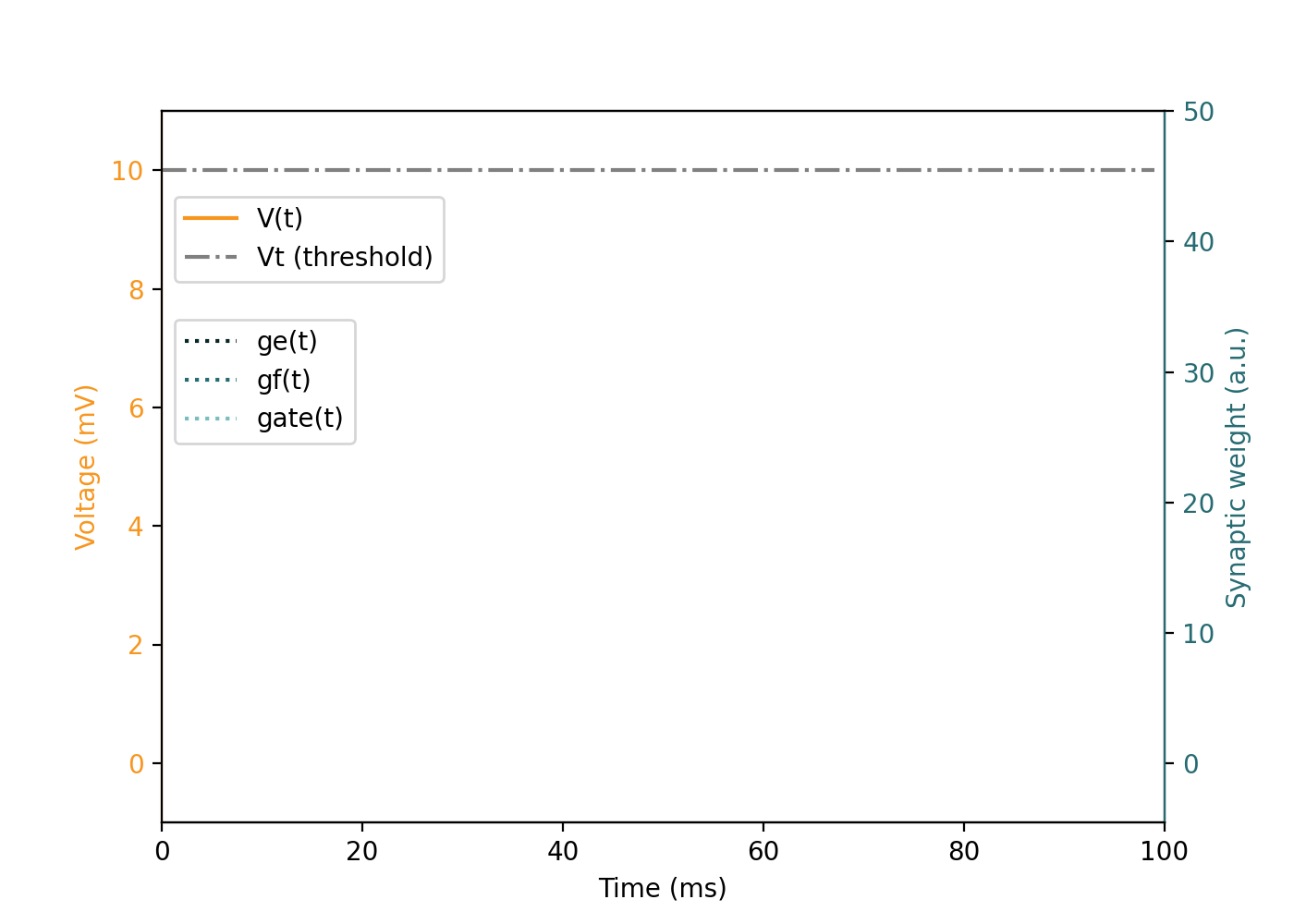
Neuron Model Animation
This animation demonstrates the evolution of an individual neuron under different synaptic inputs (V, ge, gf, gate):
| Synapse Type | Behavior |
|---|---|
V | Instantaneous jump in membrane potential V, potentially emitting spike |
ge | Slow, steady increase in V over time |
gf + gate | Fast, nonlinear voltage rise due to exponential dynamics |
gate | Controls whether gf affects the neuron at all |
Event-by-event explanation of the animation
| Time (ms) | Type | Value | Description |
|---|---|---|---|
t = 10 | V | 3.0 | Instantaneous pushes of V, membrane potential |
t = 25 | ge | 6.0 | Applies constant integration current: slow, linear voltage increase |
t = 40 | gf | 16.0 | Adds fast-decaying input, gated via gate = 1 at same time |
t = 40 | gate | 1.0 | Enables gf affecting neuron dynamics |
t = 85 | spike | - | Neuron emits a spike and resets its state |
Synapse Types
The neuron model has 4 synapse types. Each of them affects one of the 4 internal state variables of the neuron receiving the synapse. Synapses have a certain weight (w):
| Synapse Type | Effect | Explanation |
|---|---|---|
V | V += w | Immediate change in membrane potential |
ge | ge += w | Adds to the constant input |
gf | gf += w | Adds to the exponential input |
gate | gate += w | Toggles gate flag (w = ±1) to activate gf |
Besides it’s weight w, wach synapse also includes a delay, controlling the the time taken by a spike travelling through the synapse to arrive to the following neuron and affecting it’s internal state:
synapse
  | weight
  | delay
Numerical Parameters
By default, Axon uses the following numeric values for the neuron parameters
| Parameter | Numeric value (mV, ms) | Meaning |
|---|---|---|
Vt | 10.0 | Spiking threshold |
Vreset | 0.0 | Voltage after reset |
tm | 100.0 | Membrane integration constant |
tf | 20.0 | Fast synaptic decay constant |
Units are milliseconds for time values and millivolts for membrane potential values.
Benefits of This Model
This neuron model is designed for interval-coded values. Time intervals between spikes directly encode numeric values.
The neuron model has dynamic behaviours that eenable symbolic operations such as memory, arithmetic, and differential equation solving. The dynamics of this neuron model forms a Turing-complete computation framework (for in depth information, refer to the STICK paper).
This neuron model has the following characteristics:
- Compact: Minimal neurons required for functional blocks
- Precise: Accurate sub-millisecond spike-based encoding
- Composable: Modular design supports hierarchical circuits
- Hardware-Compatible: Ported to digital integrate-and-fire cores
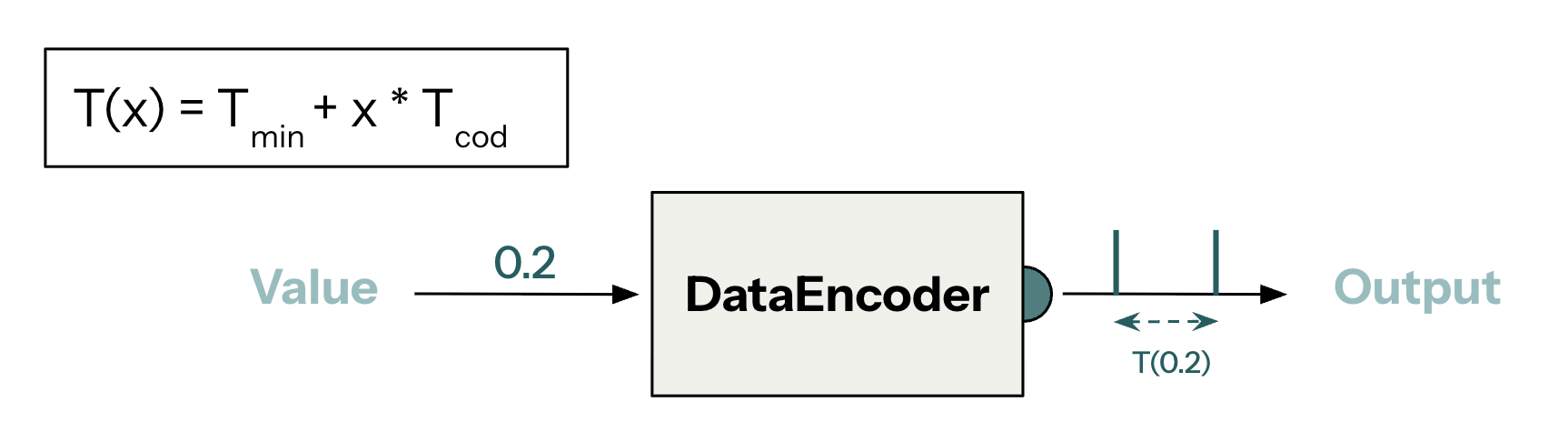
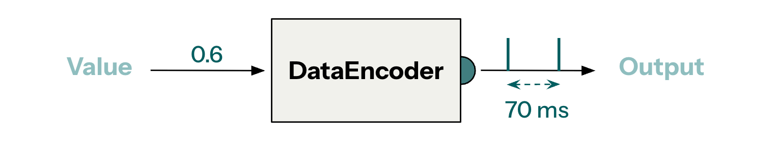
Interval Coding
Axon encodes scalars values into pairs of spikes. The time difference between the 2 spikes in a pair, also called the Inter Spike Interval (ISI), relates to the encoded value. The DataEncoder class is responsible for encoding values into spikes and decoding them back.
This document highlight how this encoding and decoding process works.
scalar values into inter-spike intervals (ISIs) and decoding them back. This functionality is central to how Axon implements symbolic computation using the STICK (Spike Time Interval Computational Kernel) framework.
This document explains how Axon implements the interval-based encoding and computation as defined by the STICK (Spike Time Interval Computational Kernel) model.
Concept
In Axon, numerical values are encoded in the time difference between two spikes. Other neuromorphic models use encoding schemes such as spike rates or voltage values. However, time-encoding has the following advantages:
- Keeps the sparsity of spike events and hence enables ultra-low power consumption.
- Allows for high numeric resolution by using time domain while keeping spikes as binary events.

Values x ∈ [0,1] are encoded in the time difference Δt between two spikes:
ΔT = Tmin + x * Tcod
x   = (ΔT − Tmin) / Tcod
where:
Tmin: minimum time differenceTcod: coding intervalΔT: time difference between two spikes
As a consequence, Tmax = Tmin + Tcod.
Default coding values are:
| Parameter | Numeric value (ms) | Meaning |
|---|---|---|
Tmin | 10.0 | Spiking threshold |
Tcod | 100.0 | Voltage after reset |
Tmax | 110.0 | Membrane integration constant |
Example:
ΔT(0.6) = 10 ms + 0.6 * 100 ms = 70 ms
Interval-based Computation
Spiking networks are built to process interval-encoded values. The network dynamics are governed by the synaptic weights and delays, allowing for complex computations based on the timing of spikes.
- Value
xis represented by timing between spikes Δt. - Spiking networks manipulate these intervals via synaptic delays, integration, and gating, executing operations like addition, multiplication, and memory.
DataEncoder Class
The DataEncoder class provides methods for encoding and decoding values:
class DataEncoder:
    def __init__(self, Tmin=10.0, Tcod=100.0):
        ...

    def encode_value(self, value: float) -> tuple[float, float]:
        ...

    def decode_interval(self, spiking_interval: float) -> float:
        ...
The DataEncoder is used during simulation and output processing:
from axon_sdk.simulator import Simulator
from axon_sdk.encoders import DataEncoder

encoder = DataEncoder(Tmin=10.0, Tcod=100.0)
spike_pair = encoder.encode_value(0.6)
spike_pair
>> (0.0, 70.0)
This spike pair can then be injected into the network, and the simulator will handle the timing based on the encoded intervals.
sim.apply_input_value(value=0.6, neuron=input_neuron)
Output Decoding
interval = spike_pair[1] - spike_pair[0]
decoded_value = encoder.decode_interval(interval)
decoded_value
>> 0.6
Simulator engine
The Axon SDK simulates Spiking Neural Networks (SNNs) built with the STICK framework. This document describes the simulation engine’s architecture, parameters, workflow, and features.
Purpose
The Simulator class provides a discrete-time, event-driven environment to simulate:
- Spiking neuron dynamics
- Synaptic event propagation
- Interval-based input encoding and output decoding
- Internal logging of voltages and spikes
It is optimized for symbolic, low-rate temporal computation rather than high-frequency biological modeling.
from axon_sdk.simulator import Simulator
Core Components
The Simulator wraps a SNN, defined as an SpikingNetworkModule, inputs spikes to it and simulates its dynamics.
class Simulator:
    def __init__(self, net: SpikingNetworkModule, encoder: DataEncoder, dt: float = 0.001):
      ...
These are the components needed to instantiate a new simulator:
| Component | Description |
|---|---|
net | The user-defined spiking network (a SpikingNetworkModule) |
encoder | Object for encoding/decoding interval-coded values |
dt | Simulation timestep in seconds (default: 0.001) |
Calling .simulate(simulation_time) executes the simulation.
Note: It’s the user’s responsability to set an appropriate
simulation_timethat allows the SNN to finalize its dynamic evolution.
Simulation logs
The simulator logs relevant information during the simulation, which can be retrieved once it’s finished:
| Property | Description |
|---|---|
.spike_log | Dictionary mapping neurons to the timing of their emitted spikes |
.voltage_log | Dictionary mapping neurons to the evolution of their membrane potentials |
Input injection
The Simulator is responsible for inputting values to the SNN:
| Property | Description |
|---|---|
.apply_input_value(value, neuron, t0) | Encodes a value and inputs their corresponding spikes |
.apply_input_spike(neuron, t) | Inputs an individual spike |
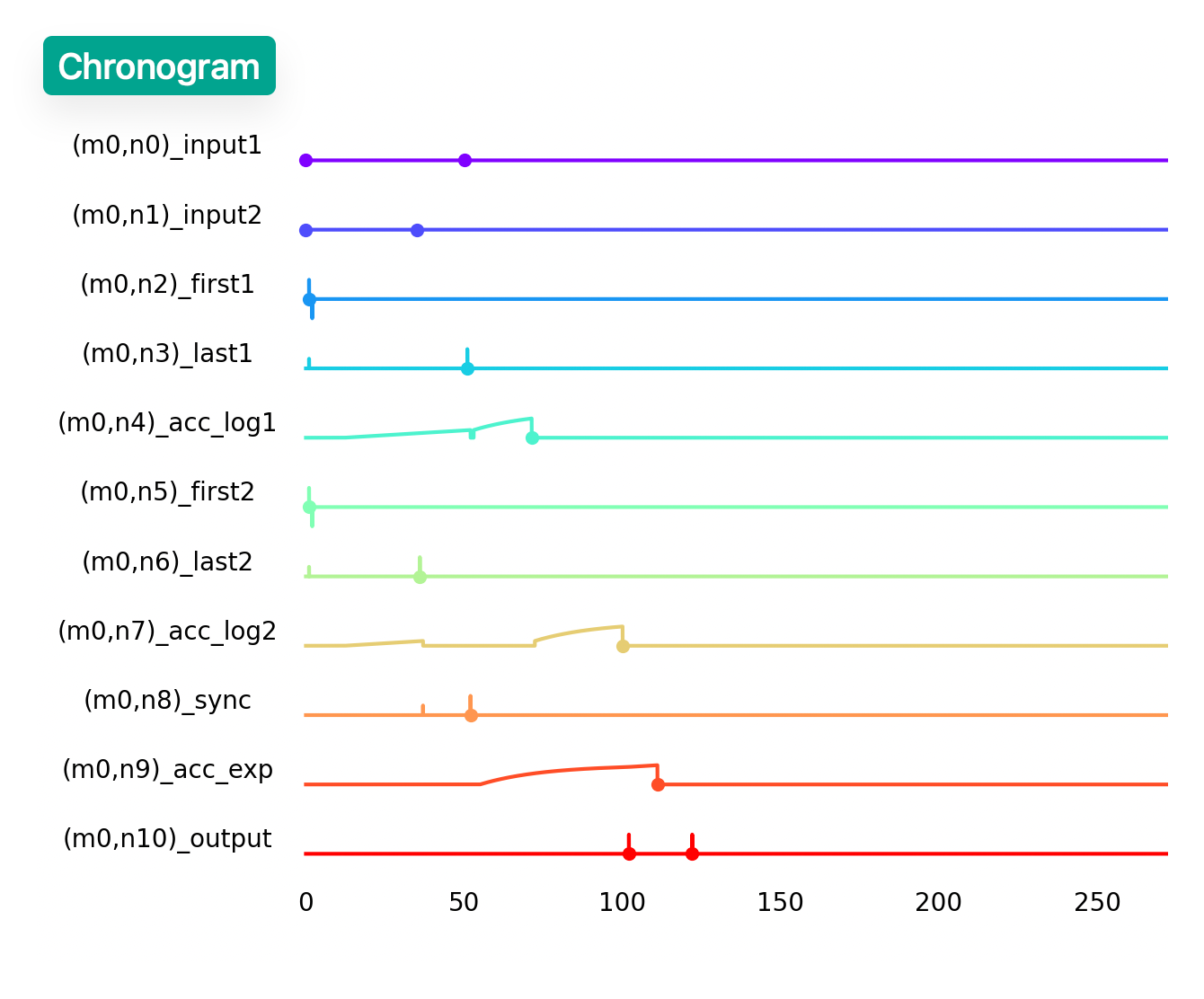
Visualization
Axon provides visualization tools for debugging purposes:
- Network topology visualization
- Chronogram
These visualizations are shown once the simulation is done.
To enable the visualization tools, the environment variable VIS must be set
| Environment Variable | Description |
|---|---|
VIS=1 | Opens visualization after simulation |
Usage example:
VIS=1 python mul_network.py
Example usage
from axon_sdk.simulator import Simulator
from axon_sdk.networks import MultiplierNetwork
from axon_sdk.primitives import DataEncoder

encoder = DataEncoder()
net = MultiplierNetwork(encoder)
sim = Simulator(net, encoder, dt=0.001)

a, b = 0.4, 0.25
sim.apply_input_value(a, net.input1, t0=0)
sim.apply_input_value(b, net.input2, t0=0)
sim.simulate(simulation_time=400)

spikes = sim.spike_log.get(net.output.uid, [])
interval = spikes[1] - spikes[0]
decoded_val = encoder.decode_interval(interval)
decoded_val
>> 0.1
Summary
- Event-driven, millisecond-resolution simulator
- Supports interval-coded STICK networks
- Accurate logging of all internal neuron dynamics
- Integrates seamlessly with compiler/runtime interfaces
About
About and contact
Axon SDK is a neuromorphic framework to build spiking neural networks (SNN) for general-purpose computation.
Axon SDK was build by Neucom. At Neucom, we’re building a general-purpose neuromorphic processor that executes deterministic computation tasks with minimal energy consumption.
![]()
Axon SDK is based on the theoretical work presented in STICK and it expands it in several directions:
- Axon SDK provides a library of spiking computation kernels that can be combined to achieve complex computations.
- Axon SDK extends STICK with an arbitrary computation range, beyond the original constrain to scalars in the [0, 1] range.
- Axon SDK provides new computation primitives, such as a Modulo operation, Scalar multiplication and Division.
- Axon SDK provides a compiler that translates a user-defined algorithms using Python syntax syntax, into their spiking version.
- Axon SDK includes a Simulator to emulate the operation of the constructed SNN.
Axon SDK is open-sourced under a GPLv3 license, preventing its inclusion in closed-source projects.
Axon SDK was developed by Iñigo Lara, Francesco Sheiban and Dmitri Lyalikov and belongs to Neucom APS. Neucom APS is based in Copenhagen, Denmark.
Contact
If you’re working with Axon or STICK-based hardware and want to share your application, request features, or report issues, reach out via GitHub Issues or contact the Neucom team at francesco@neucom.ai.
![]()
Contributing
If you’d like to contribute to Axon SDK, then you should begin by forking the public repository at to your own account, commiting some code and opening a PR.
You are also welcome to submit issues to the Github repo.
We use main as a stable branch. You should commit your modifications to a new feature branch.
$ git checkout -b feature/my-feature develop
...
$ git commit -m 'This is a verbose commit message.'
Then push your new branch to your repository
$ git push -u origin feature/my-feature
Use the Black code formatter on your final commit. This is a requirement. If your modifications aren’t already covered by a unit test, please include a unit test with your merge request. Unit tests use pytest and go in the tests/ directory.
Then when you’re ready, make a merge request on Github the feature branch in your fork to the Axon SDK repo.
Building the documentation
The documentation is based on mdbook.
To build a live, locally-hosted HTML version of the docs, use the following commands (you’ll need to install Rust and mdbook):
cd axon-sdk
mdbook serve --open
The docs are built automatically as part of our CI/CD pipeline when a new commit arrives to main.
Running the tests
As part of the merge review process, we’ll check that all the unit tests pass. You can check this yourself (and probably should), by running the unit tests locally.
To run all the unit tests for Axon SDK, use pytest:
cd axon-sdk
pytest tests
The test are run automatically as part of our CI/CD pipeline in every branch.
References
Axon SDK is based on theoretical work proposed in the following paper by Xavier Lagorce and Ryad Benosman:
Xavier Lagorce, Ryad Benosman; STICK: Spike Time Interval Computational Kernel, a Framework for General Purpose Computation Using Neurons, Precise Timing, Delays, and Synchrony. Neural Comput 2015; 27 (11): 2261–2317. doi: https://doi.org/10.1162/NECO_a_00783